Artificial Intelligence 🤖, Machine Learning ⚙, and Others 🌌

The paper is concerned with beliefs about future performances of securities and the construction of a portfolio which can maxmimise returns.

Markowitz is not convinced that an investor can maximize returns without taking variance into consideration or without diversifying their portfolio. Hence he introduces the expected returns-variance (\( E \)-\( V \)) rule.

The \( E \)-\( V \) rule states that the investor would (or should) want to select one of the portfolios with the minimum \( V \) for a given \( E \) or a maximum \( E \) for a given \( V \). No where in the paper is it proven that diversification is necessary; it is taken as a given based on observations.

Using known statistics and probablity theory rules and the assumption that there won't be any short sales, he states the expected return \( E \) and variance \( V \) of a portfolio consisting of \( N \) securities as \[ E = \sum_{i=1}^{N} X_i \mu_i \tag{1} \] \[ V = \sum_{i=1}^{N} \sum_{j=1}^{N} \sigma_{ij} X_i X_j \tag{2} \] \[ \sum X_i = 1 \tag{3} \] \[ X_i \ge 0 \tag{4} \] where,

\( X_i \) is the percentage of the investor's assets allocated to the \( i^{\text{th}} \) security,
\( \mu_i \) is the expected value of the \( i^{\text{th}} \) security,
\( \sigma_{ij} \) is the covariance between the returns of the \( i^{\text{th}} \) and \( ^{\text{th}} \) security,
\( X_j \) is the percentage of the investor's assets allocated to the \( j^{\text{th}} \) security,

Definitions

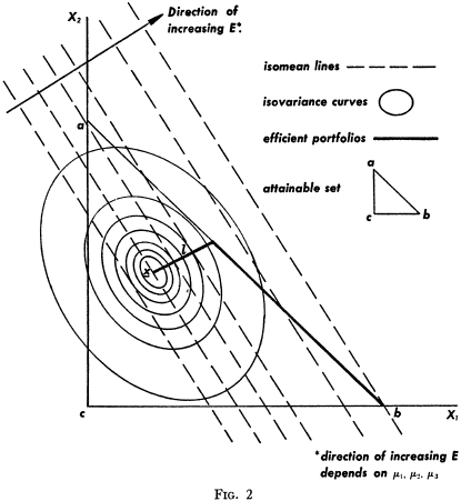
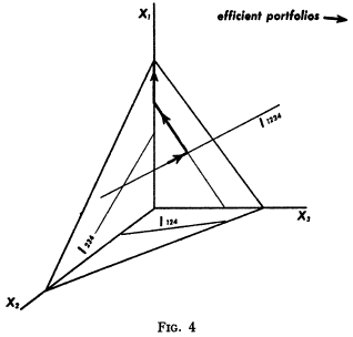
• Attainable set: of portfolios consists of all portfolios which satisfy (3) and (4).


• Isomean curve: is the set of all points (portfolios) with a given expected return; are usually a system of parallel lines.


• Isovariance line: is the set of all points (portfolios) with a given variance of return; are usually a family of concentric ellipses.


• X: is the center of the above system of isovariance ellipses which denotes minimal variance \( V \).


• Critical line: is the locus of points that minimise variance for each given expected return \( E \).

Attainable and efficient \( \boldsymbol{E} \), \( \boldsymbol{V} \) combinations

By combining statistical techniques and the judgement of experts to form reasonable probability beliefs (\( \mu_i, \sigma_{ij} \)), the above figure of attainable \( E \), \( V \) combinations can be charted.

Number of securities=3, \( \boldsymbol{X} \) inside the attainable set

The point on any isomean line at which it has a minimal variance is the point where it is tangent to any isovariance curve. If we start plotting all these points, we have the efficient line \( l \) starting from \( X \) toward the boundary. This constitutes the efficient set, which after hitting the boundary starts extending downwards towards \( b \) which is the maximum attainable \( E \).

Number of securities=3, \( \boldsymbol{X} \) outside the attainable set, critical line cuts admissible area

The efficient line begins at the attainable point with minimum variance, on the \( \overline{ab} \) line. It moves towards \( b \) until it intersects the critical line, moving along the critical line until it intersects a boundary and finally moves along the boundary to \( b \).

Number of securities=4

The efficient set is a series of connected line segments, at one end of which is the point of minimum variance and at the other end is a point of maximum expected return.

Number of securities = 3, nature of the set of efficient \( E \), \( V \) combinations

\( E \) is a plane and \( V \) is a paraboloid. As shown in Fig 5., the section of the \( E \)-plane over the efficient portfolio set is a series of connected line segments. The section of the \( V \)-paraboloid over the efficient portfolio set is a series of connected parabola segments. If we plotted \( V \) against \( E \) for efficient portfolios, we would again get a series of connected parabola segments as seen in Fig. 6.

Portfolio consisting of 2 portfolios with equal variance

If two portfolios have equal variance then typically the variance of the resulting (compound) portfolio will be less than the variance of either original portfolio. This is illustrated in Fig. 7 which can be interpreted by noting that a portfolio \( P \) which is built out of two portfolios \( P' = (X_1', X_2') \) and \( P'' = (X_1'', X_2'') \) is of the form $$ P = \lambda P' + (1 - \lambda) P'' = (\lambda X_1' + (1 - \lambda) X_1'',\ \lambda X_2' + (1 - \lambda) X_2''). $$ \( P \) is on the straight line connecting \( P' \) and \( P'' \).

In closing

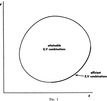
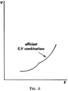
The \( E \)-\( V \) principle can be used in theoretical analysis or in the actual selection of portfolios.

If used in the selection of securities, statistical computation can be used to arrive a tentative set of \( \mu_i \) and \( \sigma_{ij} \). One way of arriving at a tentative set is to use the observed \( \mu_i \), \( \sigma_{ij} \) for some period in the past.

Judgement could then be used in increasing or decreasing some of these \( \mu_i \) and \( \sigma_{ij} \) on the basis of factors or nuances not taken into account by the formal computations. Using this revised set of \( \mu_i \) and \( \sigma_{ij} \), the set of efficient \( E \), \( V \) combinations can be computed, the investor can select the combination they prefer, and the portfolio which gives rise to this \( E \), \( V \) combination can be found.